Gradient–Operator Networks and Ordered Constraint Formation Across Scales
Abstract
Organized structure across physical, biological, and cosmological systems emerges when energetic gradients interact with structural constraints that restrict admissible system trajectories.
Developmental Constraint Theory (DCT) formalizes this interaction as an ordered sequence in which gradients are captured by structural operators and propagated through distributed constraint networks.
Across domains—including crystal lattices, photonic materials, fluid circulation systems, biological sensing systems, and cosmological structure formation—the same architecture appears:
gradients enter structured systems → constraint geometry restricts trajectories → energy redistributes through nested operator networks.
This framework provides a unified structural description of how ordered constraint formation produces persistent, organized system behavior.
The Gradient–Constraint Problem
Energetic gradients are ubiquitous:
They arise from:
- radiation fields
- thermodynamic differences
- pressure gradients
- electrochemical potentials
- gravitational fields
However, gradients alone do not produce organized systems.
Activation occurs only when a structural operator enables admissible coupling between system state space and environmental forcing :
Without this condition, gradients dissipate rather than organize.
Structural Operators and Admissibility
Structural operators (Δ) are physical architectures that allow gradients to enter a system and interact with its internal states.
Examples include:
- crystal lattice geometries
- membrane ion channels
- receptor complexes
- photonic interference structures
- neural transduction systems
System definition:
Admissible interaction requires:
Ordered Constraint Formation (SACCADE)
DCT formalizes system development as an ordered sequence:
- Signal — non-zero gradient
- Arrival — coupling via structural operator
- Context — environmental constraint conditions
- Constraint — restriction of admissible trajectories
- Adaptation — parameter reconfiguration
- Distribution — propagation across the system
- Evolution — structural reorganization
This ordering is required for persistent system formation.
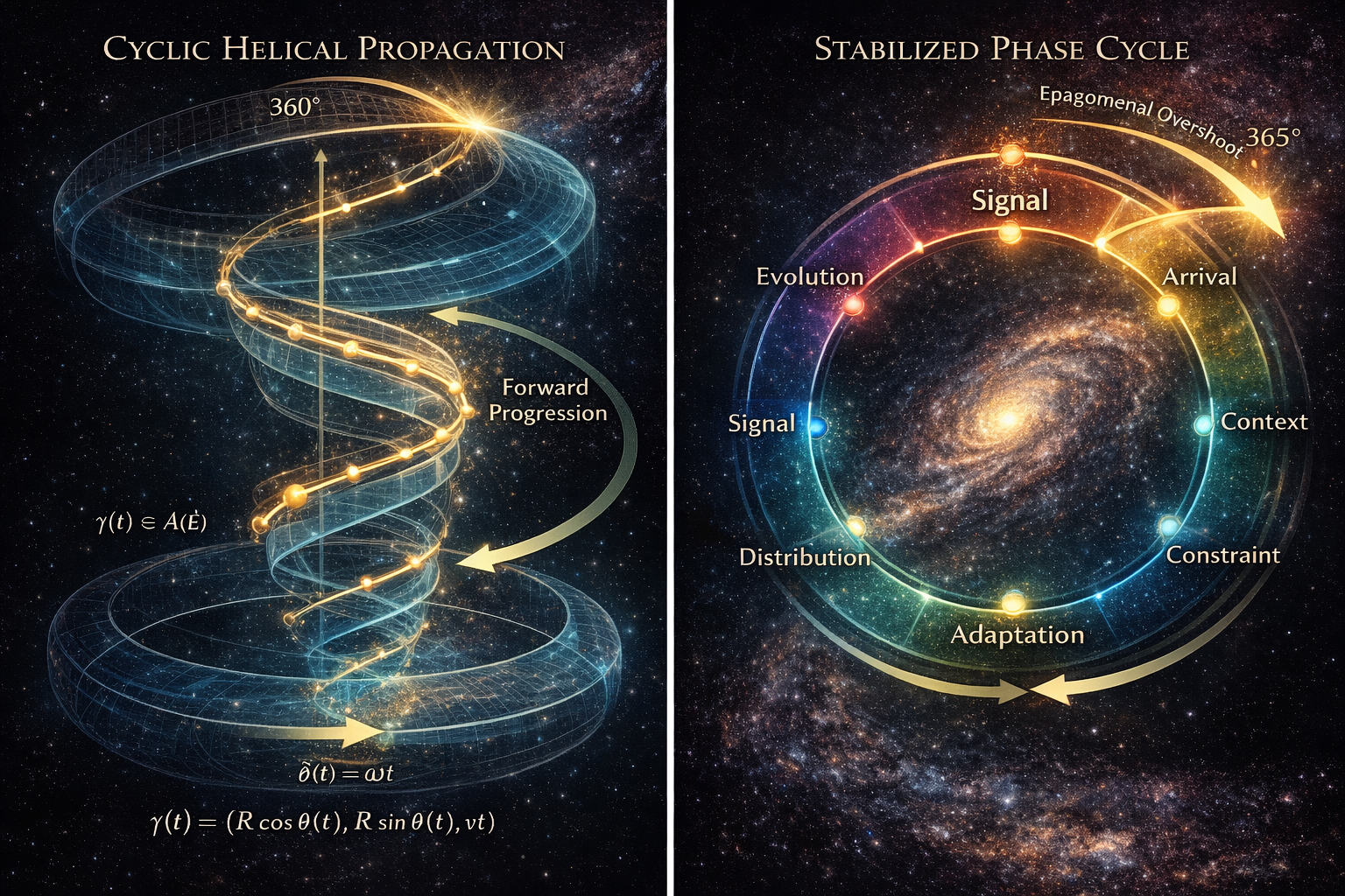
Residual states generated at cycle completion enable admissible coupling between systems.
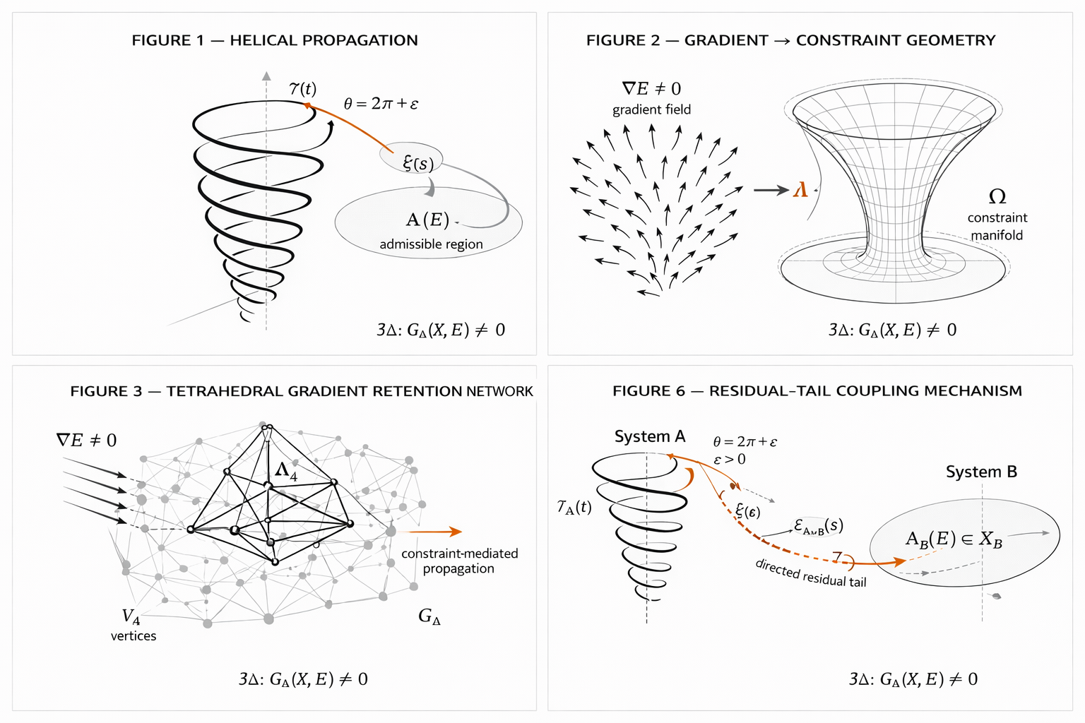
Constraint Geometry: Tetrahedral Retention Networks
This represents a 3-simplex: A recurring structure across domains is the tetrahedral coupling architecture:
- 4 vertices
- 6 edges
- 4 faces
It forms the minimal stable architecture for distributed gradient retention.
Key properties:
- maximal connectivity in 3D
- energetic stability
- infinite lattice propagation
This structure appears in:
- silicate minerals
- carbon bonding
- DNA backbone coordination
- crystal lattices
These networks distribute gradients while preventing collapse.
Nested Operator Architecture
Systems are not single-layered. They consist of nested operators:
- Outer operator: captures environmental gradients
- Inner operator: redistributes energy through recurrence
This produces:
capture → constraint → recurrence → redistribution
Persistence requires:
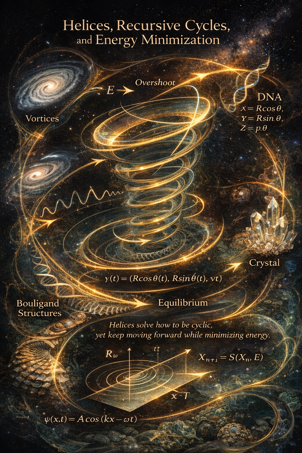
Recurrence and Helical Propagation
Many systems exhibit cyclic behavior with forward progression.
This produces a helical trajectory:
- cycles repeat locally
- system state advances globally
This defines recursive, non-reset system behavior.
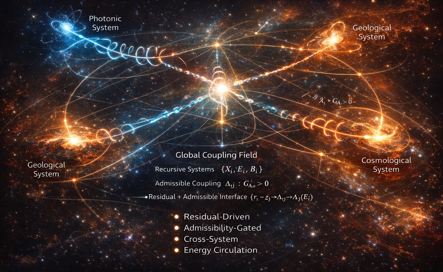
Global Coupling Field
Energy propagates across nested systems:
This produces a global coupling field in which:
- gradients are captured
- redistributed
- transferred across systems
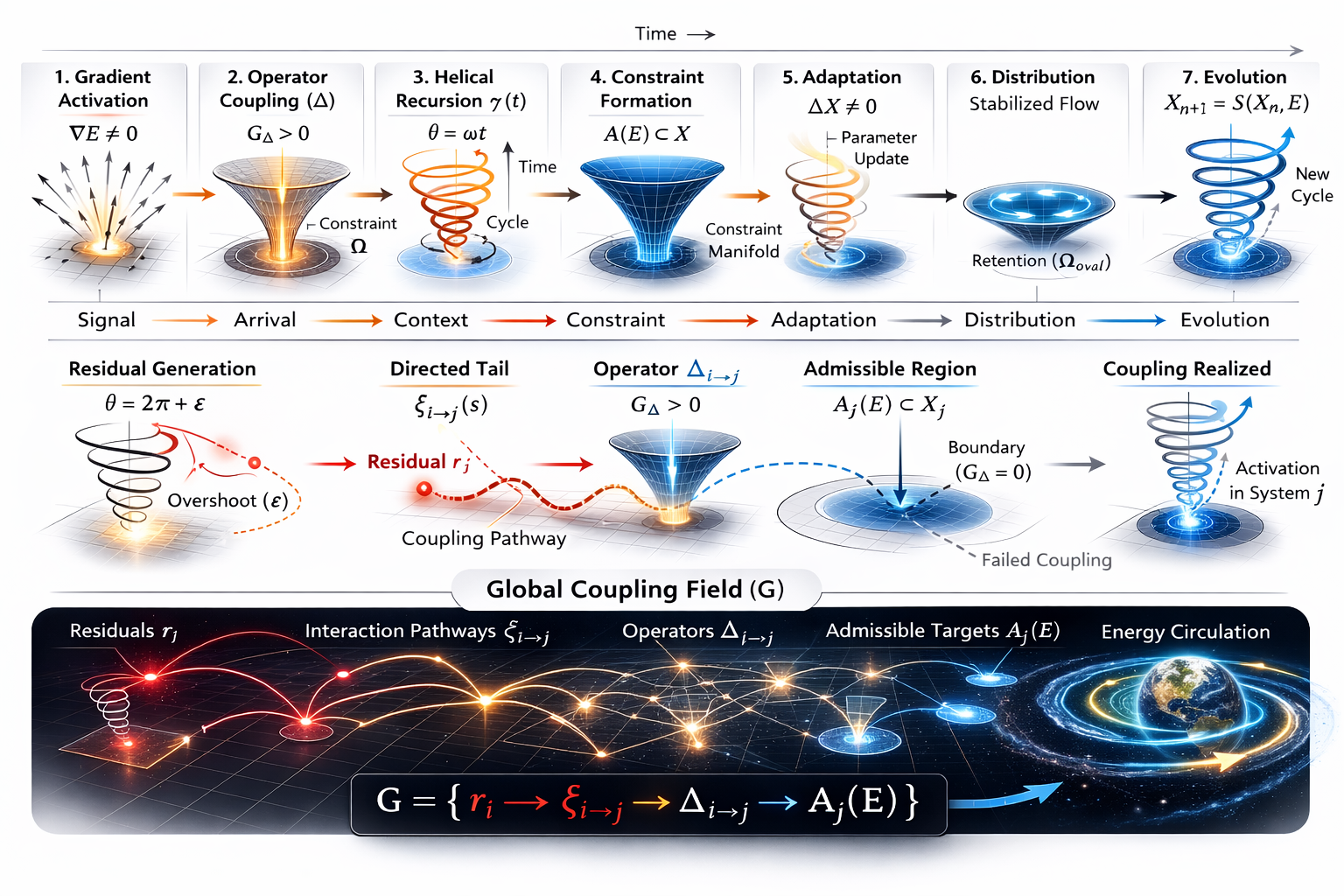
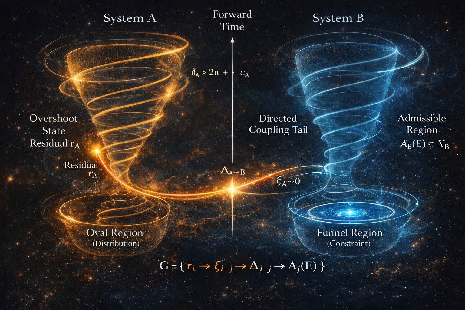
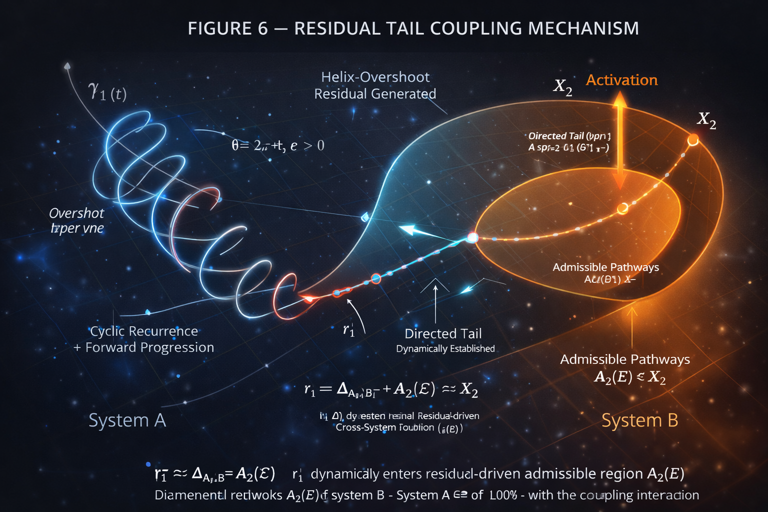
Overshoot and Cross-System Coupling
Cycles do not terminate exactly at closure:
This overshoot generates a residual:
Residual states enable cross-system coupling:
Coupling occurs only when:
This produces recursive system activation across domains.
Recursive System Dynamics
System evolution follows a recursive operator:
within a constrained manifold:
This recursion is measurable via a Poincaré return map:
The system forms a bounded helical attractor, not an infinite loop.
Cross-Domain Expression
This architecture appears across:
- mineral growth and crystal formation
- mantle convection and plate tectonics
- ocean and atmospheric circulation
- photonic biological systems
- neural signal transduction
- planetary and galactic structure
Across all cases:
gradients + constraint geometry → persistent structured systems
Structural Conclusion
Developmental Constraint Theory proposes that organized structure emerges when gradients interact with constraint architectures that restrict system trajectories.
Across all domains, the same ordered structure appears:Signal→Arrival→Context→Constraint→Adaptation→Distribution→Evolution
Persistent systems arise not from gradients alone, but from distributed operator networks that sustain admissible coupling across scales.
